 CogniDev
2 · How a codebase is read
How the workbench reads your code
One pass over the repository produces everything the rest of the product uses. This section covers what that pass works out, how it is stored, how it decides which code can be reached, and the views you get on top of it.
The structural pass
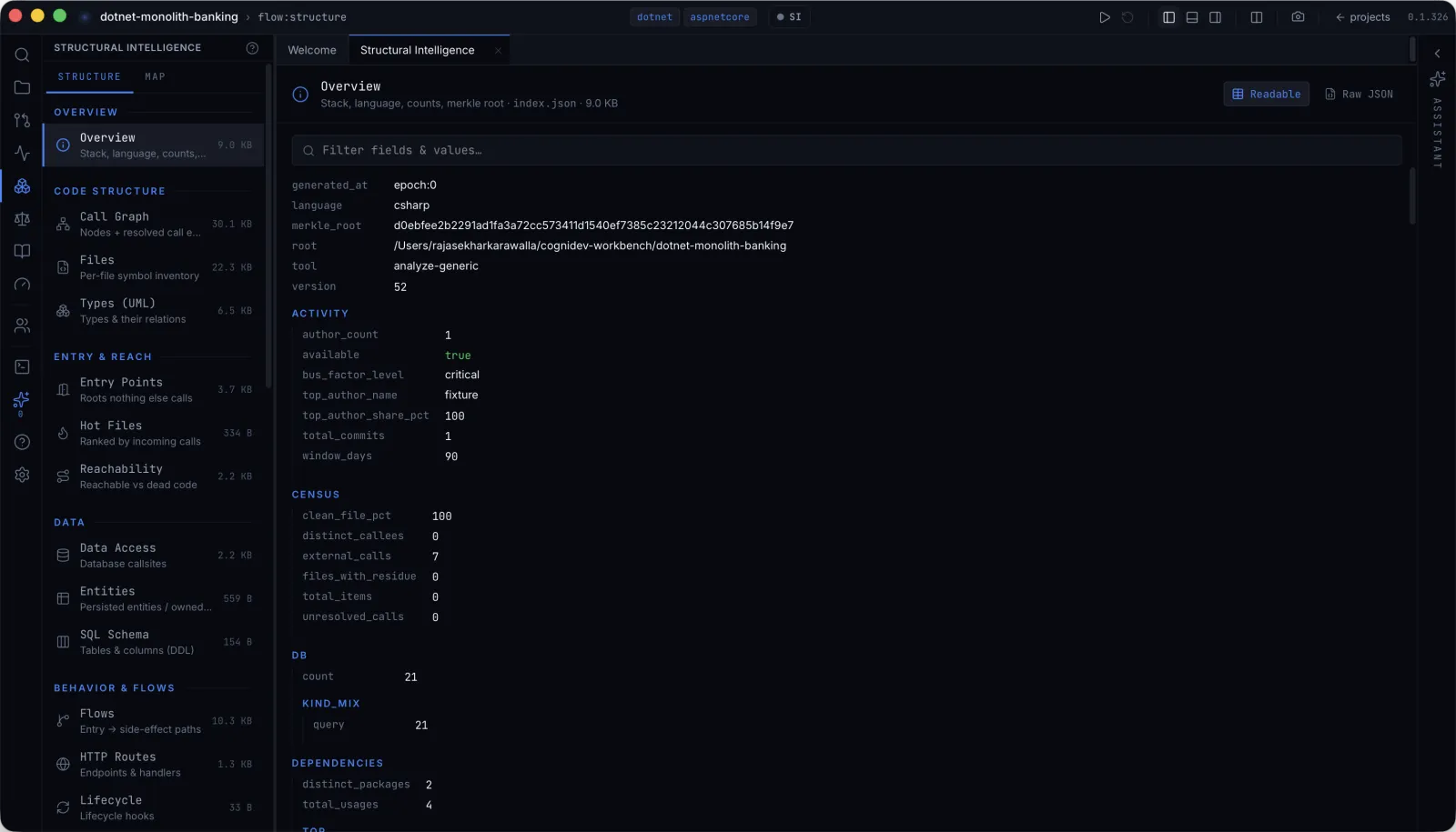
One analysis runs over the repository. It writes a set of JSON files, called shards, that describe the code from different angles: what each file declares, which function calls which, where the program starts, what it asks the database for, which HTTP routes exist, and so on.
Every screen in the product reads those shards. The views below, the governance score, the Modernize screen and the planning step of any run all work from the same pass. None of them re-reads your source.
The same code gives the same result
The overview shard carries a merkle_root, a checksum over the tree
that was analysed. The same source always produces the same value, and changing one
file changes it. That is what lets the analysis be cached and compared. A later run
can tell what actually moved instead of redoing everything, and two machines looking
at the same commit agree on what they are looking at.
It sits in your working tree
The shards are written to .cognidev/ next to the code. You can read
them formatted or as raw JSON, filter them by field or value, and commit them with the
repository if you want your team to have them.
What the pass produces
The shards are grouped the way the product groups them. Which ones you get depends on the repository. A project with no SQL has no schema shard, and the polyglot and test shards only show up where they apply.
| Group | Shards |
|---|---|
| Overview | Stack, language, counts, merkle root |
| Code Structure | Files, with what each one declares · Call Graph, with the calls it could resolve · Types, as UML · Structural Graph, with resolved calls, writes and handles plus infrastructure |
| Entry & Reach | Entry Points · Reachability · Hot Files |
| Data | Entities and the tables they own · Database call sites · SQL schema from the DDL |
| Behaviour & Flows | Flows, from an entry point to a side effect · State Map · Sequences · HTTP Routes · Roles and authorization · Lifecycle hooks |
| Architecture | Layers · Domains · Folder summaries · Dependencies · Graph insights, meaning centrality, cycles and clusters · Modules, per runtime |
| Packages & Framework | Framework API, with the real package signatures |
| Test Automation | Selenium suite: page objects, selectors, data injection |
| Product & Docs | Use Cases · Reading Guide · Logs · Screens · Locator, a search index for finding where something is · Repos · Activity |
Each row shows how big the shard is, which is a quick way to see how much of that thing the repository actually has. A large call graph next to a tiny hot-files shard describes a very different system from the other way round.
Entry points and reachability
Two shards do more than their size suggests.
Entry points are the places nothing else calls, which is where execution actually starts. Reachability walks the call graph out from those points and marks what can be reached.
That is what makes the dead-code count trustworthy instead of a guess. A file with nothing pointing at it is not necessarily dead, because it might be an entry point. A file that is referenced can still be unreachable, if everything referencing it is unreachable too. You need the entry points and the graph together to answer the question, and both are worked out from the code rather than guessed from how things are named.
The same walk produces hot files, ranked by how many calls come into them. Between them, the three tell you where to start reading, what is safe to delete, and what will be expensive to change.
Evidence and confidence
Findings come with the thing that produced them. The Tech Stack view shows this most clearly.
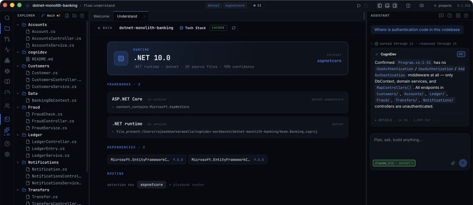
The runtime is given as .NET 10.0, from 20 source files, at 90 per cent confidence. The confidence figure is part of the finding, so you can decide how much weight to give it.
Under each framework is the evidence.
content_contains:Microsoft.AspNetCore means that text was found in the
source. file_present:…/Acme.Banking.csproj means that file is on disk.
Neither is an opinion, and you can check both by hand in a few seconds.
The same page shows the key that decides which runs get offered for this
repository, here aspnetcore. So you can see why a particular set of runs
shows up later, at the point the stack was decided.
What it could not read
The second rule is about what the analysis could not do.
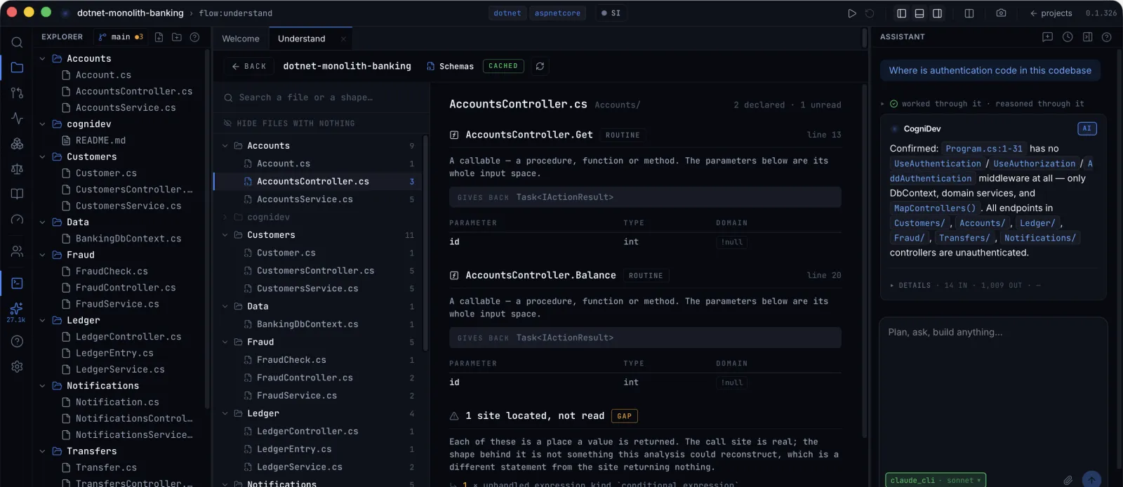
The Schemas view lists every signature and response shape the pass captured. The row worth looking at is at the bottom: a call site that is real, but whose shape the analysis could not work out. It is marked as a gap, and the screen says plainly that a gap is not the same as the call site returning nothing.
This matters more than it sounds. A tool that quietly drops what it failed to parse produces a clean-looking report that covers less of the system than you think. Here you can see what was missed, so a plan built on the analysis carries the same caveat, and you know which parts of it rest on complete information.
The same rule applies to runs
When a run cannot confirm one of its own checks from what it read, it says so instead of marking it passed. There is an example in Upgrading a .NET application in place.
Finding your way around
Understand it gives you a set of views rather than one report. Each card shows the count it found, so you can see the shape of the repository before opening anything.
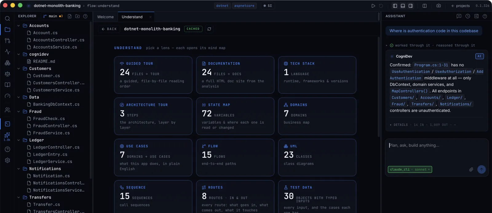
These four answer the first question anyone has on a codebase they do not know: what is this, and where do I start reading?
| View | What it shows |
|---|---|
| Guided tour | The files in a sensible reading order, in chapters. Where to start, and what to read next. |
| Documentation | A full documentation site built from the analysis and written to .cognidev/docs/. No model is involved, so it costs nothing and cannot drift away from the code it was built from. |
| Tech Stack | Runtime, frameworks and versions, each with its evidence and a confidence figure. |
| Architecture tour | The architecture one layer at a time. |
The two tours are different on purpose. One walks the files in reading order, the other walks the layers. On a repository you do not know, start with the first.
What the system does
These views describe what the system does, rather than how it is arranged.
| View | What it shows |
|---|---|
| Domains | The business areas in the code and what sits in each. |
| Use Cases | What the application does, in plain English, with the files that do it. |
| Flow | Paths from an entry point through to a side effect. |
| Sequence | Call sequences, as diagrams. |
| State Map | Module-level variables and where each one is read or changed. |
| Lifecycle | How each entity moves through its states. This only appears when at least one entity has a status to move through, so an application without one never shows it. |
Use cases in more detail
This is the view that reads the system as a product rather than a program.
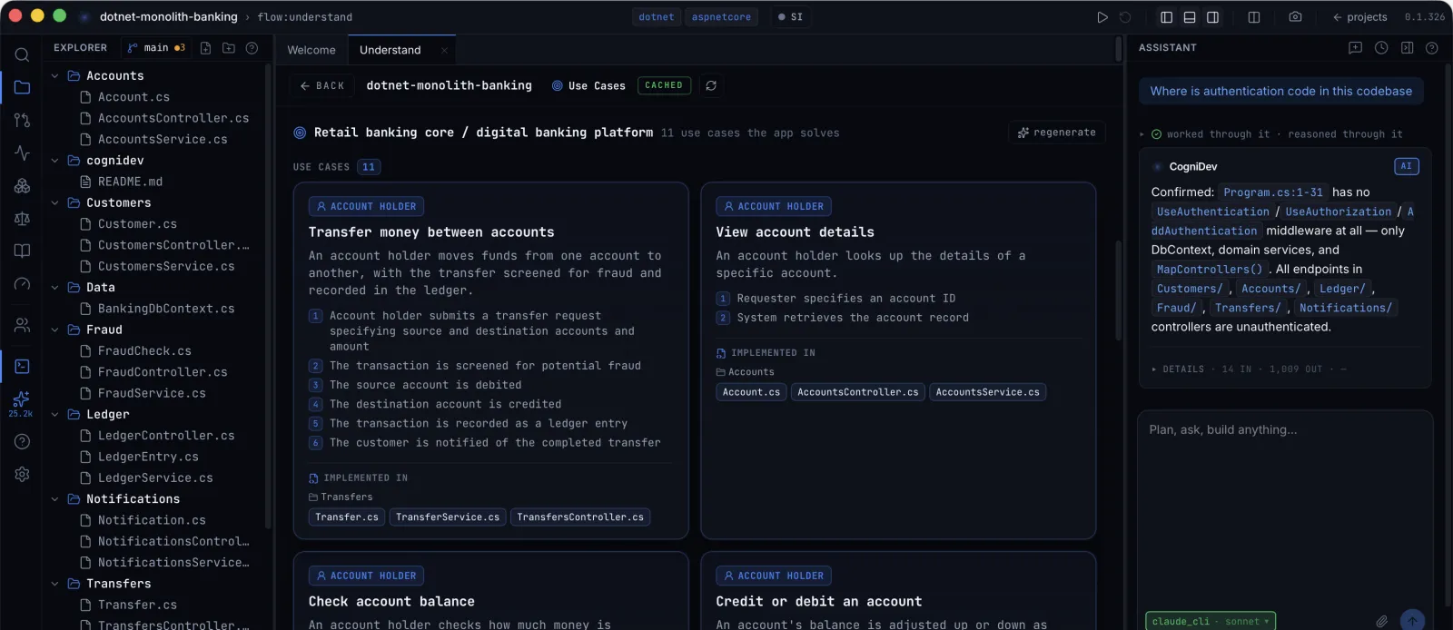
A retail banking core comes out as eleven use cases. Each is broken into the steps it actually performs. A transfer is submitted, screened for fraud, debited, credited, recorded, and the customer is told. Each step names the files that do the work.
That helps with two jobs. Someone new starts from what the system does rather than from the folder names. And when an audit asks where a business rule lives, you have a file to open instead of a search to run.
Contracts and data
These views cover what crosses the boundary and what the data behind it looks like.
| View | What it shows |
|---|---|
| Routes | Every route: what goes in, what comes out, and what it touches. |
| Data Model | Typed fields, the values each one can hold, and the test data those values imply. |
| Schemas | Open a file and see every object, payload and schema declared inside it. |
| Stored Procedures | Every routine: its signature, what it declares, the tables it touches, and what it does. Shown where the repository has stored routines. |
| Test Data | Every typed input, and the cases each one has. |
Data Model and Schemas show the same information from opposite ends. Data Model starts with a type and tells you what it holds. Schemas starts with a file and tells you what is declared inside it, which is the question you have when you are looking at one. Which is more useful depends on what you already know.
Test Data exists because a typed input with known limits already tells you what its cases are. The view does not invent values. It works out what the declared types allow.
Structure and risk
These views cover how the code is wired together, and where it is likely to hurt.
| View | What it shows |
|---|---|
| UML | Class diagrams from the types that were parsed. |
| Insights | Hotspots, cycles and clusters, from the call graph. |
| Wiring | Routes, infrastructure, and how far a change can reach. Needs a structural graph for the runtime, which today means Go, Java, JavaScript, Python and Rust. |
| Map | Browse the files and see what flows in and out of each one. |
| Dependencies | The outside packages you use, and where each one is used. |
| Dead code | Files nothing can reach, worked out from the entry points and the call graph. |
| Tests | The shape of the test suite itself. Shown where the project has a Selenium suite. |
How far a change reaches
Insights and Wiring answer the question that decides how big a change really is. Insights ranks files by how central they are, so the file everything depends on gets named up front instead of found later. Wiring follows the call graph out from a change to show what it can reach.
Empty is an answer
A view with nothing in it says so in its own words: "Nothing unreachable — all files are reachable", or "No Selenium suite in this project". An empty result and an unsupported one never look the same.